Are you looking for information on how to examine your scKaryo-seq data? This post will introduce you to the basics of scKaryo-seq analysis, enjoy!

Goal

The goal of this walk through is to aid researchers with their scKaryo-seq data analysis. In this example we will be walking through some techniques and tools which can be used to visualize genetic heterogeneity within a (tumor) sample.

Data source

The sequencing data in this walk through are derived K562 myelogeneous leukemia cells. These samples were processed and sequenced using scKaryo-seq by the Single Cell Core facility at the Hubrecht Institute. Sequencing data was pre-processed using the SingleCellMultiOmics package of the Van Oudenaarden lab.

Requirements

This walk through will focus on using the Aneufinder R-package for data visualization. As such it is required to have R and R-studio as well as the necessary libraries installed.

if (!require("BiocManager", quietly = TRUE))
  install.packages("BiocManager")

BiocManager::install("AneuFinder")

BiocManager::install("BSgenome.Hsapiens.NCBI.GRCh38")

Sequencing data

The scKaryo-seq sequencing data used in this tutorial can be cloned from this page.

Cleaning up the data

When performing single cell sequencing analysis there is a very good chance that some of the cells did not yield sufficient data for further analysis. These cells will have to be removed from the data set in order to focus our efforts to those cells which meet our criteria (the “good” cells).

Setup

Start a new Rscript and load the libraries that we will be using throughout this tutorial.

library(AneuFinder)
library(BSgenome.Hsapiens.NCBI.GRCh38)

Set the working directory of your Rscript to that of your analysis directory and initialize the following variables.

######### Setup ##############

setwd("D:/Analysis") # something like that

count_table <- read.table("./count_table_1000000.csv", sep = ",", header = T)

input_folder <- "./single_cells"
output_folder <- "./karyo_results"

host_genome <- BSgenome.Hsapiens.NCBI.GRCh38
#host_genome <- BSgenome.Hsapiens.UCSC.hg38
chrom <- c(1:22,"X","Y")

Removing the “bad” cells

There are a number of manners to distinguish good from bad cells. In our example we will set a initial threshold criteria for the amount of unique reads that a single cell must meet. To accomplish this we’ll use a few functions.

#### get bad cells function ####
getbad <- function(nl, min_thr, max_thr){
  cell_list <- list()
  for (i in 1:length(nl)){
    if (nl[[i]] <= min_thr || nl[[i]] >= max_thr){
      cell_list <- c(cell_list, names(nl[i]))
    }
  }
  return(unlist(cell_list))
}

### Move file function ###

my.file.move <- function(from, to) {
  file.copy(from = from, to   = to)
  file.remove(from)
}

Set the criteria for the threshold.

######### Cell selection ###########
total_reads <- colSums(count_table[4:ncol(count_table)], na.rm = T, dims = 1)

#95th percentile
#min_cutoff <- median(total_reads) - 2 * sd(total_reads)
#max_cutoff <- median(total_reads) + 2 * sd(total_reads)

#or specify it manually
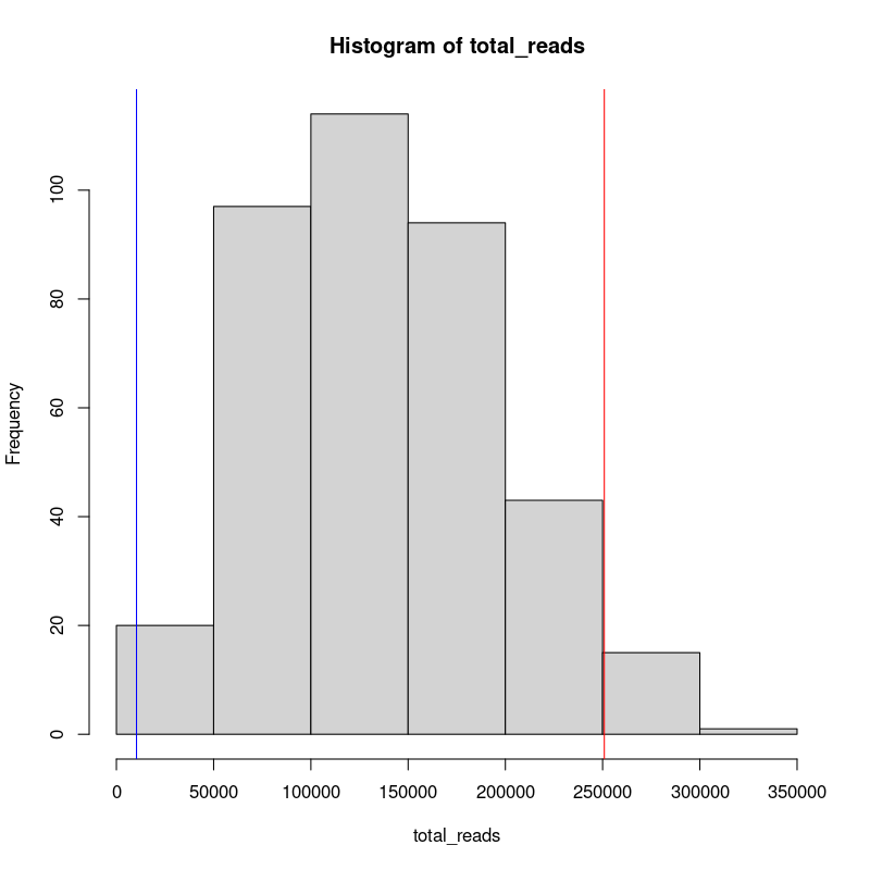
min_cutoff <- 10000
max_cutoff <- 90000

To evaluate our selection criteria it can be useful to visualize this in a histogram.

#inspect the read count distribution histogram 
png("./cell_distribution.png", width=800, height=800, res=100)
hist(total_reads)
abline(v=min_cutoff, col="blue")
abline(v=max_cutoff, col="red")
dev.off()

Once we are satisfied with our threshold, we will create a list of “undesired” cells and exclude that data from our input folder. We will then analyze the remainder of the cells.

#create a list of bad cells
bad_cells <- getbad(total_reads, min_cutoff, max_cutoff)
bad_cells <- gsub("\\.","-", bad_cells)

write.table(bad_cells, file="./bad_cells.txt", sep="\n", row.names = F, col.names = F, quote = F)

# Move sequencing data of cells with insufficient coverage.
my.file.move( from = paste0(input_folder, "/sc.", bad_cells,".bam"), 
                to = paste0(input_folder, "/insufficient_reads/sc.", bad_cells,".bam"))

my.file.move( from = paste0(input_folder, "/sc.", bad_cells,".bam.bai"), 
              to = paste0(input_folder, "/insufficient_reads/sc.", bad_cells,".bam.bai"))

AneuFinder

AneuFinder is a tool developed by Aaron Taudt to aid researchers with copy-number detection, breakpoint detection, and karyotype and heterogeneity analysis in single-cell whole genome sequencing and strand-seq data. I highly recommend having a look at their vignettes and citing their research paper when using this tool for your own research.

Mappability correction

{to/do}

Run Aneufinder

ref_bins <- "./sorted_simulated.bam"
Aneufinder(inputfolder = input_folder, outputfolder = output_folder, numCPU = 2,  pairedEndReads = F, binsizes = 1e+06, variable.width.reference = ref_bins, hotspot.pval = NULL, chromosomes = chrom, correction.method = 'GC', GC.BSgenome = host_genome, method='edivisive', cluster.plot = F)

Secondary quality controls

Once Aneufinder finished its run the outputs will be saved in the output folder. Although we initially excluded some bad cells solely based on unique read counts, we can now use the tools in Aneufinder to further examine our sample. Using clusterByQuality we are able to distinguish a number of clusters using our quality metrics.

## Get the results 
r_output <- paste0(output_folder, "/MODELS/method-edivisive")
files <- list.files(r_output, full.names=TRUE)

## Cluster by quality, please type ?getQC for other available quality measures
cl <- clusterByQuality(files, measures=c('spikiness','num.segments','entropy','bhattacharyya','sos'))
plot(cl$Mclust, what='classification')


print(cl$parameters)

For more information on the quality metrics, you may read more about them here.

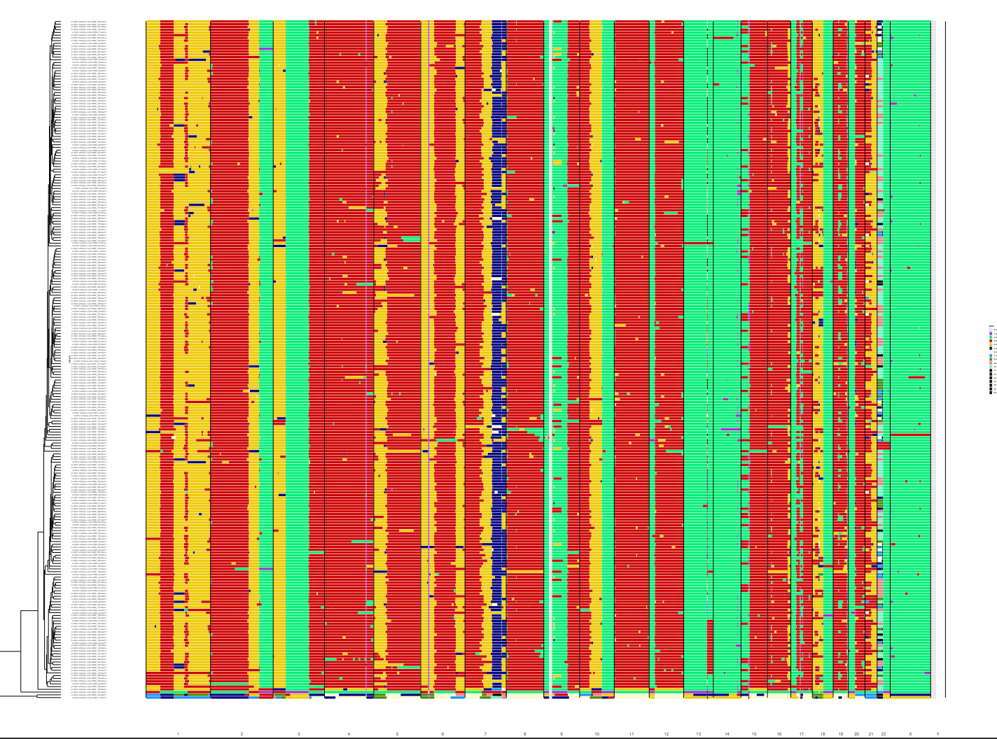
To further inspect our clusters we can produce a pdf with a heatmap for each of the clusters.

heatmapGenomewideClusters(cl, file = "./genome_heatmap_all.pdf")

For our goal we set out to visualize the tumor heterogeneity within our sample. So now we can select a cluster of interest and examine that in more detail.

## Select the best cluster and plot it separately
selected.files <- unlist(cl$classification[1]) 
heatmapGenomewide(selected.files, file="./heatmap_cl1.pdf")

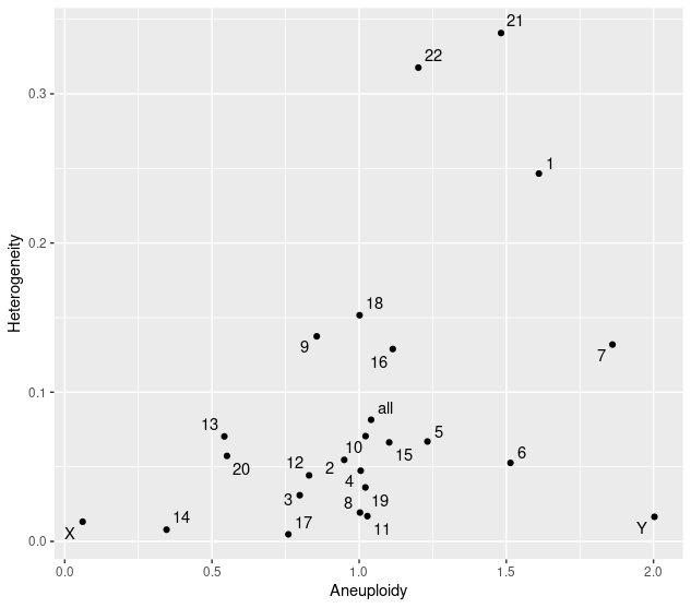
## plot Heterogeneity 
plotHeterogeneity(selected.files)

## report aneuploidy and heterogeneity scores
karyotypeMeasures(selected.files)